pacman::p_load(sf, dplyr, sfdep, spdep, mapview, tmap, plotly, tidyverse, knitr, ggplot2, spacetime)Take-home Exercise 1: A Comprehensive Spatial Pattern Analysis of Bus Passenger Trips in Singapore
Setting the Scene
In modern cities, digital transformations in transportation and public utilities, including buses, taxis, mass transit, and roads, generate extensive datasets. These datasets can track patterns of movement over time and space, especially with the widespread integration of technologies like GPS and RFID in vehicles. For instance, smart cards and GPS devices on public buses help gather data on routes and ridership. The vast amount of movement data thus collected likely reveals structural patterns and useful insights about the observed phenomena. Analyzing and comparing these patterns can offer deeper understanding of human movements and behaviors within urban environments. Such insights are valuable for enhancing city management and providing key information to both private and public urban transport service providers, aiding them in making informed decisions for a competitive edge.
However, in practical applications, the utilization of this extensive location-aware data is often limited to basic tracking and mapping using GIS (Geographic Information System) tools. This limitation stems mainly from the inadequate capabilities of traditional GIS in effectively analyzing and modeling spatial and spatio-temporal data.
Objectives
Apply Exploratory Spatial Data Analysis (ESDA) to uncover spatial and spatio-temporal mobility patterns of public bus passengers in Singapore.
Utilize Local Indicators of Spatial Association (LISA) and Emerging Hot Spot Analysis (EHSA) for this analysis.
Tasks
Task 1: Geovisualisation and Analysis
- Compute passenger trips from origin at the hexagon level during different peak hours.
| Peak hour period | Bus tap on time |
|---|---|
| Weekday morning peak | 6am to 9am |
| Weekday afternoon peak | 5pm to 8pm |
| Weekend/holiday morning peak | 11am to 2pm |
| Weekend/holiday evening peak | 4pm to 7pm |
Use appropriate geovisualisation methods to display geographical distribution of these trips.
Describe spatial patterns observed in the geovisualisations.
Task 2: Local Indicators of Spatial Association (LISA) Analysis
Calculate LISA for passenger trips by origin at hexagon level.
Display LISA maps for these trips, highlighting only significant results (p-value < 0.05).
Draw statistical conclusions based on the analysis results.
Task 3: Emerging Hot Spot Analysis (EHSA)
Conduct Mann-Kendall Test using spatio-temporal local Gi* values for passenger trips by origin at the hexagon level for the four time intervals.
Prepare EHSA maps showing Gi* values of passenger trips by origin at hexagon level, focusing on significant results (p-value < 0.05).
Describe spatial patterns revealed in EHSA maps and data visual.
1.Installing and Loading the R Packages
In the opening of our analysis, we begin by loading all the necessary packages to ensure a seamless and comprehensive analysis of spatial patterns in bus passenger trips in Singapore. The R code utilizes the pacman package for efficient package management. With pacman::p_load, we conveniently load a suite of essential packages including:
sffor handling spatial datadplyrfor data manipulationsfdepandspdepfor spatial dependenciesmapviewandtmapfor interactive mappingplotlyfor creating interactive plotstidyversefor an integrated approach to data scienceknitrfor dynamic report generationggplot2for sophisticated graphicsspacetimefor handling spatio-temporal data.
This suite of packages equips us with a robust set of tools necessary to conduct an in-depth and multifaceted analysis.
2.Data Importing and Wrangling
2.1Aspatial Data
2.1.1Importing Original Passenger Trips Data
- Passenger Volume by Origin Destination Bus Stops from LTA DataMall. In this study, we will focus on the latest data which is collected in Octomber, 2023.
Run the code chunk below to load the corresponding csv.file.
odbus <- read_csv("data/aspatial/origin_destination_bus_202310.csv")Using function glimpse() to grasp the basic structure and information of data odbus.
glimpse(odbus)Rows: 5,694,297
Columns: 7
$ YEAR_MONTH <chr> "2023-10", "2023-10", "2023-10", "2023-10", "2023-…
$ DAY_TYPE <chr> "WEEKENDS/HOLIDAY", "WEEKDAY", "WEEKENDS/HOLIDAY",…
$ TIME_PER_HOUR <dbl> 16, 16, 14, 14, 17, 17, 17, 7, 14, 14, 10, 20, 20,…
$ PT_TYPE <chr> "BUS", "BUS", "BUS", "BUS", "BUS", "BUS", "BUS", "…
$ ORIGIN_PT_CODE <chr> "04168", "04168", "80119", "80119", "44069", "2028…
$ DESTINATION_PT_CODE <chr> "10051", "10051", "90079", "90079", "17229", "2014…
$ TOTAL_TRIPS <dbl> 3, 5, 3, 5, 4, 1, 24, 2, 1, 7, 3, 2, 5, 1, 1, 1, 1…This code converts two columns ORIGIN_PT_CODE and DESTINATION_PT_CODE, into factors, which are categorical variables in R, facilitating their use in statistical modeling and analysis.
odbus$ORIGIN_PT_CODE <- as.factor(odbus$ORIGIN_PT_CODE)
odbus$DESTINATION_PT_CODE <- as.factor(odbus$DESTINATION_PT_CODE)
Check again and notice that both of them are in factor data type now.
glimpse(odbus)Rows: 5,694,297
Columns: 7
$ YEAR_MONTH <chr> "2023-10", "2023-10", "2023-10", "2023-10", "2023-…
$ DAY_TYPE <chr> "WEEKENDS/HOLIDAY", "WEEKDAY", "WEEKENDS/HOLIDAY",…
$ TIME_PER_HOUR <dbl> 16, 16, 14, 14, 17, 17, 17, 7, 14, 14, 10, 20, 20,…
$ PT_TYPE <chr> "BUS", "BUS", "BUS", "BUS", "BUS", "BUS", "BUS", "…
$ ORIGIN_PT_CODE <fct> 04168, 04168, 80119, 80119, 44069, 20281, 20281, 1…
$ DESTINATION_PT_CODE <fct> 10051, 10051, 90079, 90079, 17229, 20141, 20141, 1…
$ TOTAL_TRIPS <dbl> 3, 5, 3, 5, 4, 1, 24, 2, 1, 7, 3, 2, 5, 1, 1, 1, 1…2.2.2Extract Commuting Flow data
This code chunk below filters and summarizes the odbus data to calculate the total number of passenger trips during the weekday morning peak hours (6am to 9am). It first filters for entries on weekdays, then narrows down to entries between 6am and 9am. It groups the data by the origin point code, sums up the total trips from each origin, and replaces any missing values (NA) in the resulting trip totals with 0.
weekday_morning_peak <- odbus %>%
  filter(DAY_TYPE == "WEEKDAY") %>%
  filter(TIME_PER_HOUR >= 6 & TIME_PER_HOUR <= 9) %>%
  group_by(ORIGIN_PT_CODE) %>%
  summarise(TRIPS = sum(TOTAL_TRIPS)) %>%
  mutate(TRIPS = ifelse(is.na(TRIPS), 0, TRIPS))
This code displays the first few rows (head) of the weekday_morning_peak data frame in a well-formatted table using the kable() function, which is commonly used for creating markdown or HTML tables in R.
kable(head(weekday_morning_peak))| ORIGIN_PT_CODE | TRIPS |
|---|---|
| 01012 | 1770 |
| 01013 | 841 |
| 01019 | 1530 |
| 01029 | 2483 |
| 01039 | 2919 |
| 01059 | 1734 |
This code chunk below filters and summarizes the odbus data to calculate the total number of passenger trips during the weekday afternoon peak hours (5pm to 8pm). It first filters for entries on weekdays, then narrows down to entries between 6am and 9am. It groups the data by the origin point code, sums up the total trips from each origin, and replaces any missing values (NA) in the resulting trip totals with 0.
weekday_afternoon_peak <- odbus %>%
  filter(DAY_TYPE == "WEEKDAY") %>%
  filter(TIME_PER_HOUR >= 17 & TIME_PER_HOUR <= 20) %>%
  group_by(ORIGIN_PT_CODE) %>%
  summarise(TRIPS = sum(TOTAL_TRIPS)) %>%
mutate(TRIPS = ifelse(is.na(TRIPS), 0, TRIPS))kable(head(weekday_afternoon_peak))| ORIGIN_PT_CODE | TRIPS |
|---|---|
| 01012 | 8000 |
| 01013 | 7038 |
| 01019 | 3398 |
| 01029 | 9089 |
| 01039 | 12095 |
| 01059 | 2212 |
This code chunk below filters and summarizes the odbus data to calculate the total number of passenger trips during the weekends/holidays morning peak hours (11am to 2pm). It first filters for entries on weekends/holidays, then narrows down to entries between 11am and 2pm. It groups the data by the origin point code, sums up the total trips from each origin, and replaces any missing values (NA) in the resulting trip totals with 0.
weekend_morning_peak <- odbus %>%
  filter(DAY_TYPE == "WEEKENDS/HOLIDAY") %>%
  filter(TIME_PER_HOUR >= 11 & TIME_PER_HOUR <= 14) %>%
  group_by(ORIGIN_PT_CODE) %>%
  summarise(TRIPS = sum(TOTAL_TRIPS)) %>%
mutate(TRIPS = ifelse(is.na(TRIPS), 0, TRIPS))kable(head(weekend_morning_peak))| ORIGIN_PT_CODE | TRIPS |
|---|---|
| 01012 | 2177 |
| 01013 | 1818 |
| 01019 | 1536 |
| 01029 | 3217 |
| 01039 | 5408 |
| 01059 | 1159 |
This code chunk below filters and summarizes the odbus data to calculate the total number of passenger trips during the weekends/holidays evening peak hours (4pm to 7pm). It first filters for entries on weekends/holidays, then narrows down to entries between 4pm and 7pm. It groups the data by the origin point code, sums up the total trips from each origin, and replaces any missing values (NA) in the resulting trip totals with 0.
weekend_evening_peak <- odbus %>%
  filter(DAY_TYPE == "WEEKENDS/HOLIDAY") %>%
  filter(TIME_PER_HOUR >= 16 & TIME_PER_HOUR <= 19) %>%
  group_by(ORIGIN_PT_CODE) %>%
  summarise(TRIPS = sum(TOTAL_TRIPS)) %>%
mutate(TRIPS = ifelse(is.na(TRIPS), 0, TRIPS))kable(head(weekend_evening_peak))| ORIGIN_PT_CODE | TRIPS |
|---|---|
| 01012 | 3061 |
| 01013 | 2770 |
| 01019 | 1685 |
| 01029 | 4063 |
| 01039 | 7263 |
| 01059 | 1118 |
This code calculates the total number of bus trips for each hour on weekdays, grouped by the origin point code. It filters the odbus data for weekday entries, groups the data by origin point and hour, then sums up the trips for each group, handling missing values by removing them. Finally, it replaces any resulting missing total trip values with 0, which helps in understanding hourly variations in trip counts.
weekday_trips <- odbus %>%
  filter(DAY_TYPE == "WEEKDAY") %>%
  group_by(ORIGIN_PT_CODE, TIME_PER_HOUR) %>%
  summarise(TRIPS = sum(TOTAL_TRIPS, na.rm = TRUE)) %>%
  mutate(TRIPS = ifelse(is.na(TRIPS), 0, TRIPS))
This code calculates the total number of bus trips for each hour on weekends/holidays, grouped by the origin point code. It filters the odbus data for weekends/holidays entries, groups the data by origin point and hour, then sums up the trips for each group, handling missing values by removing them. Finally, it replaces any resulting missing total trip values with 0, which helps in understanding hourly variations in trip counts.
weekend_trips <- odbus %>%
  filter(DAY_TYPE == "WEEKENDS/HOLIDAY") %>%
  group_by(ORIGIN_PT_CODE, TIME_PER_HOUR) %>%
  summarise(TRIPS = sum(TOTAL_TRIPS, na.rm = TRUE)) %>%
  mutate(TRIPS = ifelse(is.na(TRIPS), 0, TRIPS))
This code uses the rm() function in R to remove the odbus dataset from the current R environment. This is often done to declutter the workspace and free up memory, especially when the dataset is no longer needed, thereby reducing visual distraction and potential confusion with other datasets.
rm(odbus)2.2Geospatial Data
2.2.1Importing Bus Stop Location
- Bus Stop Location from LTA DataMall: Contains information on all bus stops serviced by buses, including bus stop codes and location coordinates.
The code chunk below uses st_read() from the sf package to read the spatial data. After importing, the code transforms the spatial reference system of the bus stop data to coordinate reference system (CRS) 3414 using st_transform(), ensuring the data is in the correct format for spatial analysis within the Singapore context.
    busstop <- st_read(dsn = "data/geospatial",
                       layer = "BusStop") %>%
      st_transform(crs = 3414)
Reading layer `BusStop' from data source
`D:\KathyChiu77\ISSS624\Take-home Ex\Take-home Ex 1\data\geospatial'
using driver `ESRI Shapefile'
Simple feature collection with 5161 features and 3 fields
Geometry type: POINT
Dimension: XY
Bounding box: xmin: 3970.122 ymin: 26482.1 xmax: 48284.56 ymax: 52983.82
Projected CRS: SVY21This code is likely part of the R mapview package, which is designed to create interactive visualizations of spatial data. By calling this function with the busstop data, an interactive map is generated where each bus stop is likely represented as a point.
mapview(busstop)Looking at the map above:
The blank areas on the map where there are no purple points could represent regions without bus stops, non-residential ( like around Marina Bay) or industrial areas, parks ( like Bukit Timah Nature Reserve), or bodies of water where no bus service is.
The concentration of bus stops can give insights into urban planning, population density, and the public transport network’s reach within Singapore.
The interactive nature of the map allows users to zoom in and out to inspect areas of interest in more detail, which can be useful for both planning and analysis purposes.
2.2.2Creating the New Hexagon Layer
The code creates a hexagonal grid overlay using the st_make_grid() function applied to the busstop dataset, which contains bus stop locations in Singapore. The specified cellsize determines that each hexagon in the grid will have a diameter of approximately 577.35 meters, calculated to ensure accurate hexagonal sizing. Setting square = FALSE ensures the grid is composed of hexagons, not squares.
hex_grid <- st_make_grid(busstop, cellsize = (4/3)*sqrt(3)*250, square = FALSE)The provided code transforms the hexagonal grid into a spatial dataframe (sf object) using the st_sf() function, assigning the grid geometries as its spatial features. Subsequently, it appends a unique identifier to each hexagon by creating a new column, hex_id, with a sequence of numbers from 1 to the number of hexagons in the grid.
hex_grid_sf <- st_sf(geometry = hex_grid) %>%
  mutate(hex_id = 1:length(hex_grid))
By using the st_intersects() function, which detects the intersections between the hexagons and the bus stops, the code effectively identifies which bus stops fall within each hexagonal cell. The lengths() function is then applied to the list returned by st_intersects() to count the number of bus stops intersecting each hexagon.
hex_grid_sf$bus_stop_count <- lengths(st_intersects(hex_grid_sf, busstop))The code refines the visualization by filtering out hexagons that do not contain any bus stops.
hex_grid_sf <- filter(hex_grid_sf, bus_stop_count > 0)The code block initializes an interactive mapping mode with tmap_mode("view"), preparing for the creation of an interactive map. It then constructs the map using the tm_shape() function to specify the spatial data (hex_grid_sf) as the basis for the map. Various tm_* functions are chained together to define the map’s aesthetics and interactivity:
tm_fill: This function is used to color the hexagons based on the bus_stop_count attribute, using a blue color palette and a continuous style, with semi-transparency set byalpha = 0.6.tm_borders: Adds grey borders to each hexagon to delineate them clearly.tm_layout: Adjusts the layout, setting the legend to appear on the left bottom of the map.
tmap_mode("view")

map_hexagon <- tm_shape(hex_grid_sf) +
  tm_fill(
    col = "bus_stop_count",
    palette = "Blues",
    style = "cont",
    title = "Number of Bus Stops",
    id = "hex_id",
    showNA = FALSE,
    alpha = 0.6,
    popup.vars = c(
      "Number of Bus Stops: " = "bus_stop_count"
    ),
    popup.format = list(
      bus_stop_count = list(format = "f", digits = 0)
    )
  ) +
  tm_borders(col = "grey40", lwd = 0.7) +
  tm_layout(legend.position = c("left", "bottom"))

map_hexagonThe map visualizes the number of bus stops within each hexagonal grid cell across Singapore. The shading of the hexagons, ranging from light to dark blue, corresponds to the number of bus stops, with darker blues indicating a higher count. The darkest blue areas—Pioneer, Jurong East, Choa Chu Kang Road, Bukit Panjang Road, around Fort Canning Park and so on—suggest these are hubs with a higher density of bus stops. These locations are likely to be key transit areas that cater to significant passenger volumes due to factors like commercial activity, residential populations, and connectivity to other modes of transport. For instance, Fort Canning Park, being a popular recreational area, might also have enhanced bus services to support tourism and leisure activities.
Uses the st_write() function to save the hex_grid_sf spatial dataframe, which contains the hexagonal grid layer, to a shapefile named “hex_layer.shp” located in the “data/geospatial” directory. The append = FALSE parameter ensures that if a file with the same name already exists, it will be overwritten rather than appending the new data to the existing file.
st_write(hex_grid_sf, "data/geospatial/hex_layer.shp", append = FALSE)Deleting layer `hex_layer' using driver `ESRI Shapefile'
Writing layer `hex_layer' to data source
`data/geospatial/hex_layer.shp' using driver `ESRI Shapefile'
Writing 1237 features with 2 fields and geometry type Polygon.map_hexagon and hex_grid are removed from R environment.
rm(map_hexagon, hex_grid)3.Integrating Passenger Trips with Hexagonal Grids for Multidimensional Transit Analysis
3.1Weekday Morning Peak
To align bus stops with the corresponding hexagonal grid cells they are located in, a spatial join is executed using the st_join function from the sf package.
busstop_hex <- st_join(busstop, hex_grid_sf)This code merges two datasets: busstop_hex, which contains bus stops assigned to their respective hexagons, and weekday_morning_peak, which includes data on bus trips during weekday morning peak hours. The inner_join() function links the records based on the matching bus stop numbers (BUS_STOP_N) and origin point codes (ORIGIN_PT_CODE). The resulting weekday_morning_trips contains only the records that have a corresponding match in both dataframes, specifically for bus stops active during weekday morning peak times.
weekday_morning_trips <- busstop_hex %>%
  inner_join(weekday_morning_peak, by = c("BUS_STOP_N" = "ORIGIN_PT_CODE"))
The code is designed to identify duplicate records in the weekday_morning_trips dataframe. It groups the data by all columns using group_by_all(), then filters for groups with more than one entry using filter(n() > 1), which would indicate duplicates. After removing the grouping with ungroup(), it uses glimpse(duplicate) to provide a quick overview of the resulting dataframe. The output indicates that no rows are returned, meaning there are no duplicate entries.
duplicate <- weekday_morning_trips %>%
  group_by_all() %>%
  filter(n()>1) %>%
  ungroup()
glimpse(duplicate)
Rows: 0
Columns: 7
$ BUS_STOP_N <chr>
$ BUS_ROOF_N <chr>
$ LOC_DESC <chr>
$ hex_id <int>
$ bus_stop_count <int>
$ TRIPS <dbl>
$ geometry <GEOMETRY [m]> This code aggregates the trip data for weekday mornings by hexagon grid cells. It groups the weekday_morning_trips dataframe by hex_id (each hexagon’s unique identifier), then calculates the sum of trips for each hexagon, ensuring that any missing values (NA) are not included in the sum (na.rm = TRUE). In case there are any NA values resulting from the summarisation, it uses mutate() with ifelse to replace them with zero. The final output, hex_weekday_morning, contains the total number of trips that originated in each hexagon during weekday morning peak hours.
hex_weekday_morning <- weekday_morning_trips %>%
  group_by(hex_id) %>%
  summarise(weekday_morning_trips = sum(TRIPS, na.rm = TRUE)) %>%
  mutate(weekday_morning_trips = ifelse(is.na(weekday_morning_trips), 0, weekday_morning_trips))
The geometry column is temporarily removed from the hex_weekday_morning dataset to prepare for joining, creating a non-spatial dataframe hex_weekday_morning_df. This is done because the geometry column can sometimes complicate joins due to its complex structure.
A spatial join is then performed using inner_join from the dplyr package, which merges the trip summary data in hex_weekday_morning_df back into the hex_grid_sf spatial dataframe based on the hex_id column. This enriches the hexagon grid with the aggregated trip data, allowing for spatial analysis of trips within each hexagon.
# Remove the geometry column temporarily for the join
hex_weekday_morning_df <- hex_weekday_morning %>%
  st_set_geometry(NULL)
# Perform the join using dplyr's left_join
hex_grid_sf <- hex_grid_sf %>%
  inner_join(hex_weekday_morning_df, by = "hex_id")
The next code chunk is set to generate a static map that visualizes the distribution of weekday morning peak passenger trips across the hexagonal grid, using varying shades of blue to represent the data quantiles
tmap_mode("plot")
tm_shape(hex_grid_sf) +
  tm_fill("weekday_morning_trips",
          style = "quantile",
          palette = "Blues",
          title = "Passenger trips") +
  tm_layout(main.title = "Weekday Morning Peak Passenger Trips",
            main.title.position = "center",
            main.title.size = 1.2,
            legend.height = 0.45,
            legend.width = 0.35,
            frame = TRUE) +
  tm_borders(alpha = 0.5) +
  tm_compass(type="8star", size = 2) +
  tm_scale_bar() +
  tm_grid(alpha =0.2) +
  tm_credits("Source: LTA DataMall", position = c("left", "bottom"))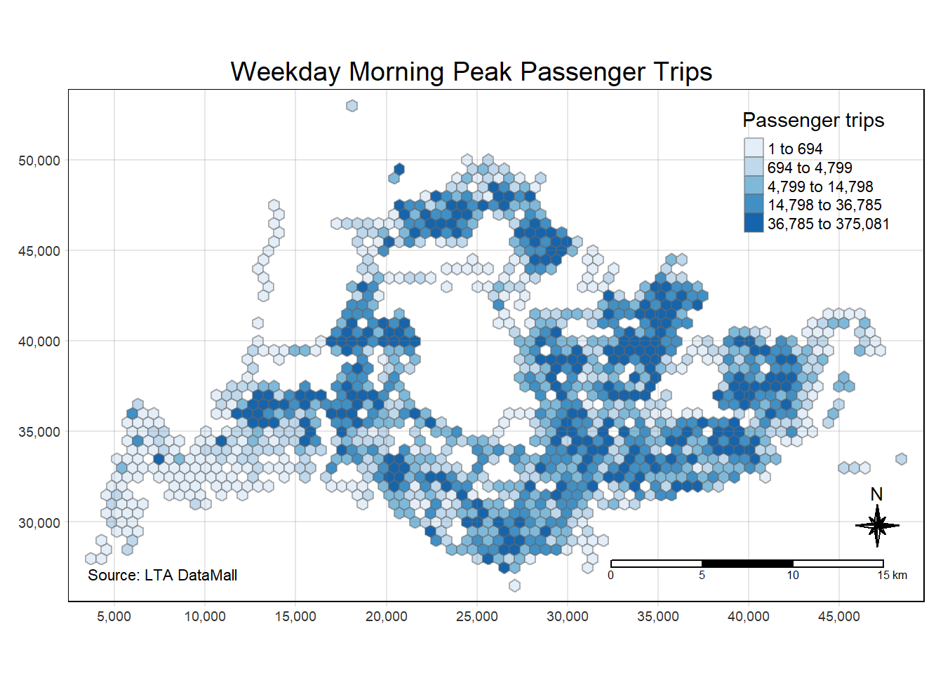
The image depicts a hexagon-based choropleth map of Singapore, illustrating the number of passenger trips made during weekday morning peak hours. From this map, we can conclude that there are significant variations in public bus usage across different areas. High-density areas, likely to be central and suburban commercial or residential hubs, show a larger number of trips, indicating these are key focus areas for transit services. Lighter shaded areas may correspond to less populated or industrial regions with fewer bus trips.
3.2Weekday Afternoon Peak
For weekday afternoon peak hours, the weekday_afternoon_trips dataframe is created by merging busstop_hex with data on afternoon trips, connecting bus stops to their trip counts using an inner join.
weekday_afternoon_trips <- busstop_hex %>%
  inner_join(weekday_afternoon_peak, by = c("BUS_STOP_N" = "ORIGIN_PT_CODE"))
For weekday afternoon trips, the code checks for duplicates in the weekday_afternoon_trips dataframe, and confirms there are none.
duplicate <- weekday_morning_trips %>%
  group_by_all() %>%
  filter(n()>1) %>%
  ungroup()
glimpse(duplicate)
Rows: 0
Columns: 7
$ BUS_STOP_N <chr>
$ BUS_ROOF_N <chr>
$ LOC_DESC <chr>
$ hex_id <int>
$ bus_stop_count <int>
$ TRIPS <dbl>
$ geometry <GEOMETRY [m]> The hex_weekday_afternoon data sums up afternoon trips for each hexagon on weekdays, replacing any missing data with zeros.
hex_weekday_afternoon <- weekday_afternoon_trips %>%
  group_by(hex_id) %>%
  summarise(weekday_afternoon_trips = sum(TRIPS, na.rm = TRUE)) %>%
  mutate(weekday_afternoon_trips = ifelse(is.na(weekday_afternoon_trips), 0, weekday_afternoon_trips))
The hex_weekday_afternoon dataframe is joined with the spatial grid, merging afternoon trip data based on hexagon IDs.
# Remove the geometry column temporarily for the join
hex_weekday_afternoon_df <- hex_weekday_afternoon %>%
  st_set_geometry(NULL)

# Perform the join using dplyr's left_join
hex_grid_sf <- hex_grid_sf %>%
  inner_join(hex_weekday_afternoon_df, by = "hex_id")
A map will display the weekday afternoon peak trips, shaded in blue to show the number of passengers.
tm_shape(hex_grid_sf) +
  tm_fill("weekday_afternoon_trips",
          style = "quantile",
          palette = "Blues",
          title = "Passenger trips") +
  tm_layout(main.title = "Weekday Afternoon Peak Passenger Trips",
            main.title.position = "center",
            main.title.size = 1.2,
            legend.height = 0.45,
            legend.width = 0.35,
            frame = TRUE) +
  tm_borders(alpha = 0.5) +
  tm_compass(type="8star", size = 2) +
  tm_scale_bar() +
  tm_grid(alpha =0.2) +
  tm_credits("Source: LTA DataMall", position = c("left", "bottom"))
The afternoon peak map for weekdays indicates a different pattern of passenger trips across Singapore compared to the morning peak. Notably, the overall trip counts appear to be higher in the afternoon, as suggested by a greater prevalence of darker blues, possibly due to people returning from work or school. The central areas remain highly active during both time slots, reflecting consistent transit usage in these urban hubs. However, there is a visible increase in activity in the outskirts in the afternoon, suggesting a movement of people towards residential areas after the workday. This contrast may reflect Singapore’s daily work commute patterns, with morning peaks focused on entry into commercial districts and afternoon peaks dispersing towards suburban residential zones.
3.3Weekend Morning Peak
The weekend_morning_trips dataframe compiles weekend morning data by joining busstop_hex with morning trip information, ensuring each bus stop’s weekend activity is accounted for.
weekend_morning_trips <- busstop_hex %>%
  inner_join(weekend_morning_peak, by = c("BUS_STOP_N" = "ORIGIN_PT_CODE"))
In the weekend_morning_trips dataframe, the same method ensures no trip entries are repeated for weekend mornings.
duplicate <- weekend_morning_trips %>%
  group_by_all() %>%
  filter(n()>1) %>%
  ungroup()
glimpse(duplicate)
Rows: 0
Columns: 7
$ BUS_STOP_N <chr>
$ BUS_ROOF_N <chr>
$ LOC_DESC <chr>
$ hex_id <int>
$ bus_stop_count <int>
$ TRIPS <dbl>
$ geometry <GEOMETRY [m]> Weekend morning trips are totaled in hex_weekend_morning for each hexagon, with missing values set to zero.
hex_weekend_morning <- weekend_morning_trips %>%
  group_by(hex_id) %>%
  summarise(weekend_morning_trips = sum(TRIPS, na.rm = TRUE)) %>%
  mutate(weekend_morning_trips = ifelse(is.na(weekend_morning_trips), 0, weekend_morning_trips))
For weekend mornings, trip summaries are integrated into the spatial grid through a join on hex_weekend_morning.
# Remove the geometry column temporarily for the join
hex_weekend_morning_df <- hex_weekend_morning %>%
  st_set_geometry(NULL)

# Perform the join using dplyr's left_join
hex_grid_sf <- hex_grid_sf %>%
  inner_join(hex_weekend_morning_df, by = "hex_id")
The weekend morning peak trips will be depicted on a map with a blue gradient indicating trip frequencies.
tm_shape(hex_grid_sf) +
  tm_fill("weekend_morning_trips",
          style = "quantile",
          palette = "Blues",
          title = "Passenger trips") +
  tm_layout(main.title = "Weekend & Holiday Morning Peak Passenger Trips",
            main.title.position = "center",
            main.title.size = 1.2,
            legend.height = 0.45,
            legend.width = 0.35,
            frame = TRUE) +
  tm_borders(alpha = 0.5) +
  tm_compass(type="8star", size = 2) +
  tm_scale_bar() +
  tm_grid(alpha =0.2) +
  tm_credits("Source: LTA DataMall", position = c("left", "bottom"))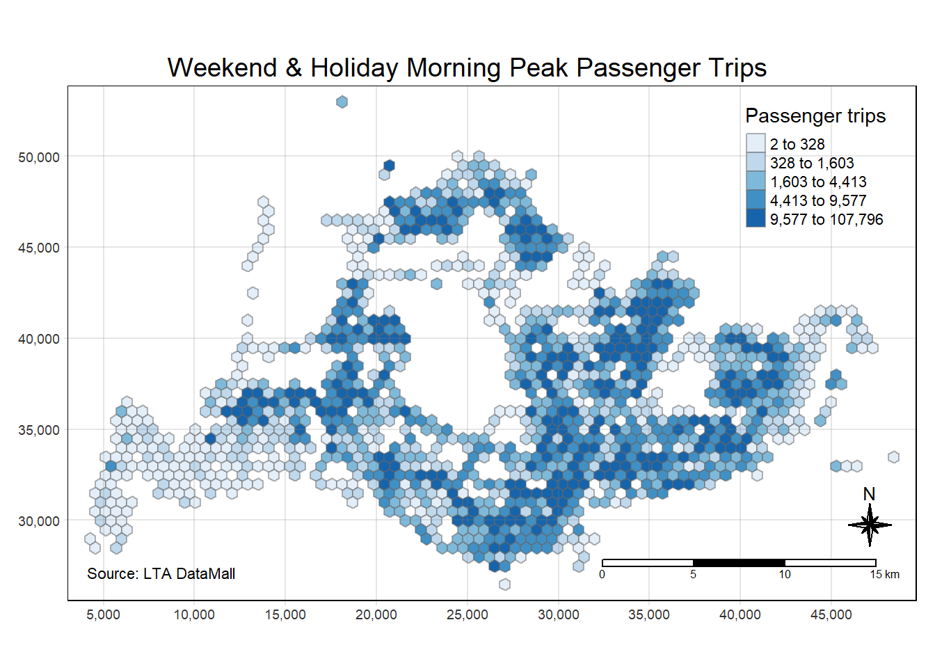
The map for weekend & holiday morning peak passenger trips in Singapore exhibits a distinct distribution when compared to the weekday morning. The range of trip counts is generally lower, as evidenced by fewer areas with the darkest shade of blue, which could be indicative of a reduced volume of commuters traveling to work or school. There appears to be a more uniform spread of medium-density travel across the island, possibly reflecting leisure or non-work-related travel patterns. The decreased intensity in central business districts and increased activity in residential or recreational areas highlight a shift in transit use, corresponding with the non-working nature of weekends in Singapore.
3.4Weekend Evening Peak
weekend_evening_trips brings together busstop_hex and data on evening bus trips during the weekend, combining the datasets to reflect each hexagon’s bus stop usage.
weekend_evening_trips <- busstop_hex %>%
  inner_join(weekend_evening_peak, by = c("BUS_STOP_N" = "ORIGIN_PT_CODE"))
Similarly, the weekend_evening_trips dataframe is verified to be free of duplicates for bus trips in the weekend evenings.
duplicate <- weekend_evening_trips %>%
  group_by_all() %>%
  filter(n()>1) %>%
  ungroup()
glimpse(duplicate)
Rows: 0
Columns: 7
$ BUS_STOP_N <chr>
$ BUS_ROOF_N <chr>
$ LOC_DESC <chr>
$ hex_id <int>
$ bus_stop_count <int>
$ TRIPS <dbl>
$ geometry <GEOMETRY [m]> hex_weekend_evening compiles the evening trip counts for each hexagon on weekends, accounting for and correcting any missing entries.
hex_weekend_evening <- weekend_evening_trips %>%
  group_by(hex_id) %>%
  summarise(weekend_evening_trips = sum(TRIPS, na.rm = TRUE)) %>%
  mutate(weekend_evening_trips = ifelse(is.na(weekend_evening_trips), 0, weekend_evening_trips))
Evening trip data for the weekend is combined with the hexagonal grid in the hex_weekend_evening dataframe using a similar join method.
# Remove the geometry column temporarily for the join
hex_weekend_evening_df <- hex_weekend_evening %>%
  st_set_geometry(NULL)

# Perform the join using dplyr's left_join
hex_grid_sf <- hex_grid_sf %>%
  inner_join(hex_weekend_evening_df, by = "hex_id")
For the weekend evening, a map will illustrate passenger trips with blue shades reflecting the volume of travel.
tm_shape(hex_grid_sf) +
  tm_fill("weekend_evening_trips",
          style = "quantile",
          palette = "Blues",
          title = "Passenger trips") +
  tm_layout(main.title = "Weekend & Holiday Evening Peak Passenger Trips",
            main.title.position = "center",
            main.title.size = 1.2,
            legend.height = 0.45,
            legend.width = 0.35,
            frame = TRUE) +
  tm_borders(alpha = 0.5) +
  tm_compass(type="8star", size = 2) +
  tm_scale_bar() +
  tm_grid(alpha =0.2) +
  tm_credits("Source: LTA DataMall", position = c("left", "bottom"))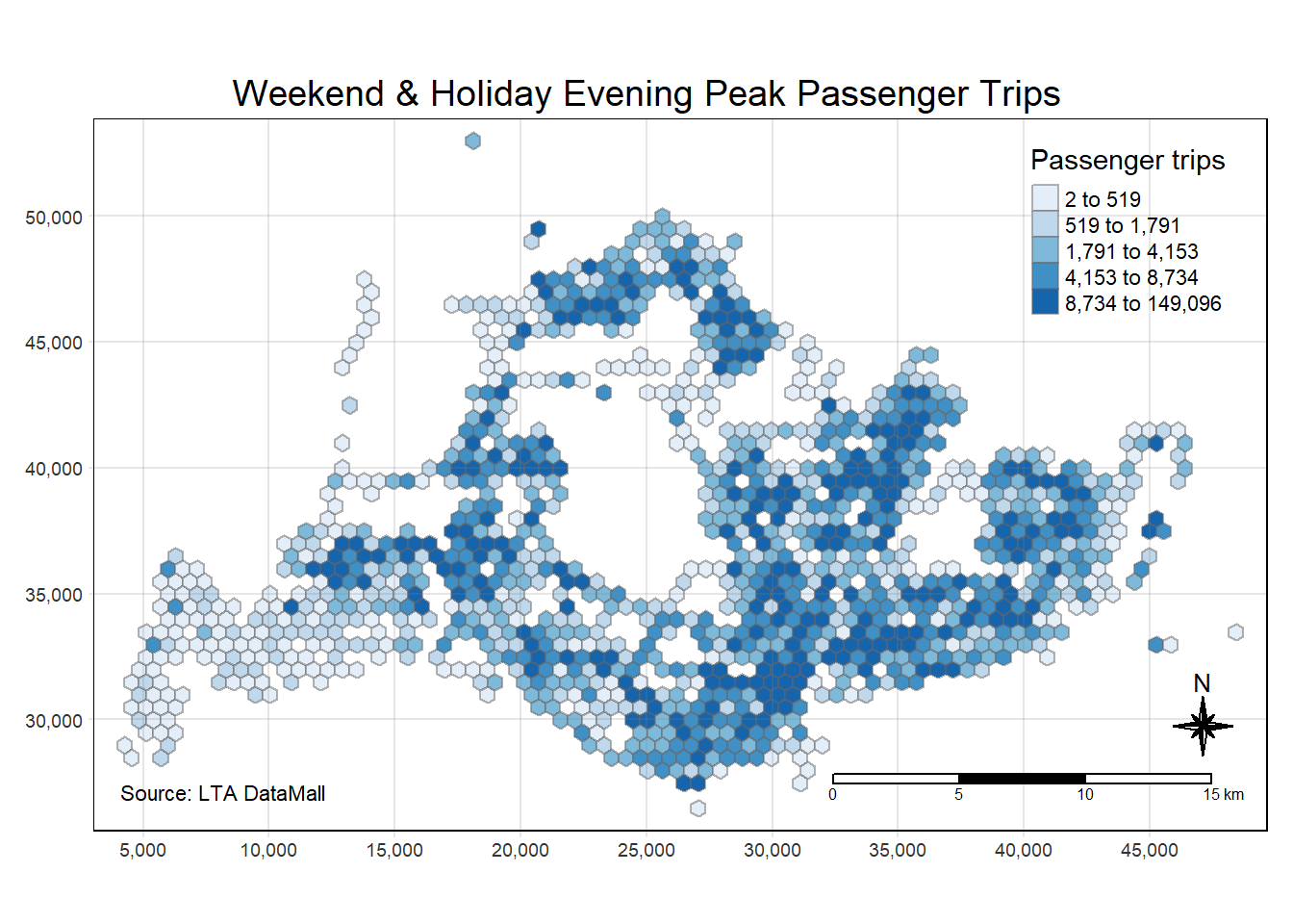
The weekend and holiday evening peak passenger trip map for Singapore reveals a different dynamic compared to the weekday afternoon. The trip densities are more evenly distributed across the island, with fewer areas of intense dark blue, which may reflect a more recreational or social travel pattern as opposed to the work-related commutes seen on weekdays. There’s also a notable presence of trips in areas that could be associated with leisure destinations or residential areas, which aligns with typical weekend and holiday evening activities. The lighter shades in the central business district areas suggest a lower volume of commuter traffic compared to the bustling weekday afternoons. This shift highlights the transition from work-focused movement to more leisurely and dispersed travel behavior in the evenings of weekends and holidays in Singapore.
The code provided is removing a list of data frames and variables related to various analyses of bus trips during different times of the day and week. By executing this command, the user is clearing the R environment of these specific objects, which helps declutter the workspace, potentially freeing up memory, and makes it easier to focus on the remaining data and analyses without the distraction of no longer needed datasets.
rm(hex_weekday_afternoon, hex_weekday_morning, hex_weekend_evening, hex_weekend_morning, hex_weekday_afternoon_df, hex_weekday_morning_df, hex_weekend_evening_df, hex_weekend_morning_df, weekday_afternoon_peak, weekday_afternoon_trips, weekday_morning_peak, weekday_morning_trips, weekend_evening_peak, weekend_evening_trips, weekend_morning_peak, weekend_morning_trips)4.Local Indicators of Spatial Association (LISA) Analysis
In the context of spatial analysis for the provided hexagonal grid, using contiguity weights can prove to be impractical, as there may be hexagons with zero neighbors, particularly on the fringes of the study area or in regions with sparse data coverage. This lack of contiguous neighbors would lead to inaccuracies in the analysis, as these hexagons would be isolated from the rest of the spatial network. Therefore, adopting a distance-based weights matrix is a more robust approach, as it accounts for the spatial relationships between hexagons based on distance rather than mere adjacency. This method ensures that all hexagons, regardless of their neighbor count, are integrated into the analysis, providing a more comprehensive understanding of the spatial dynamics at play.
4.1Deriving Fixed Distance Weights
The provided code snippet is for calculating a fixed distance weight matrix in spatial analysis. It first retrieves the spatial geometry of each hexagon from the hex_grid_sf data frame. Then, it identifies the nearest neighbors for each hexagon using a k-nearest neighbors search, which is appropriate for longitude-latitude data as indicated by the longlat = TRUE parameter. Lastly, it calculates and extracts the distances between each hexagon and its neighbors into a single vector, laying the groundwork for constructing a weight matrix based on these distances.
geo <- sf::st_geometry(hex_grid_sf)
nb <- st_knn(geo, longlat = TRUE)
dists <- unlist(st_nb_dists(geo, nb))
The first code chunk displays a summary of the dists vector, which contains the distances between each hexagon and its nearest neighbors. These statistics describe the range and central tendency of the distances, which is important for understanding the spread and typical distance between neighbors in the grid (especially the maximum 4358.9m).
summary(dists) Min. 1st Qu. Median Mean 3rd Qu. Max.
577.4 577.4 577.4 584.1 577.4 4358.9 The code chunk is creating a fixed distance weights matrix for the hex_grid_sf spatial data. The mutate() function is used to add two new columns: nb, which stores the neighbors within a certain distance band specified by the upper parameter (in this case, 4359 meters), and wt, which calculates the weights for these neighbors. The st_dist_band function is used to identify neighbors within the specified distance band, and st_weights computes the weights based on this neighbor relationship. The .before = 1 argument indicates that the new columns should be added before the first column in the existing data frame.
wm_fd <- hex_grid_sf %>%
  mutate(nb = st_dist_band(geometry,
                           upper = 4359),
               wt = st_weights(nb),
               .before = 1)
4.2Deriving Adaptive Distance Weights
The given code creates an adaptive weights matrix using the hex_grid_sf spatial data frame, which contains the geometry of a hexagonal grid. By invoking the st_knn() function with k=6, it identifies the six nearest hexagons to each hexagon as neighbors, forming an adaptive neighborhood structure that does not rely on a fixed distance. Subsequently, the st_weights() function calculates the weights for these k-nearest neighbor relationships. The new neighbor and weight columns are added to the beginning of the data frame. This adaptive method is particularly useful for ensuring each hexagon is evenly connected to a set number of neighbors, which is beneficial for spatial analyses in heterogeneous areas.
wm_ad <- hex_grid_sf %>%
  mutate(nb = st_knn(geometry,
                     k=6),
         wt = st_weights(nb),
               .before = 1)
4.3Calculate Inverse Distance Weights
The code snippet provided outlines the steps to create an inverse distance weights (IDW) matrix for the hex_grid_sf spatial dataframe, which contains the geometries of a hexagonal grid. The process begins by establishing contiguity-based neighbors for each hexagon using the st_contiguity() function, which assesses adjacency between features. Following this, the st_inverse_distance() function is applied to generate weights that are inversely proportional to the distance between neighbors—meaning that closer neighbors have greater influence than those farther away. The scale parameter is set to 1, maintaining the original distance units, and alpha is set to 1, indicating that the weight will be the reciprocal of the distance. These weights are then inserted at the start of the dataframe. The resulting wm_idw dataframe contains an IDW matrix which captures the intensity of spatial relationships based on proximity, suitable for spatial analyses where the effect of distance is expected to diminish with increasing separation.
wm_idw <- hex_grid_sf %>%
  mutate(nb = st_contiguity(geometry),
         wts = st_inverse_distance(nb, geometry,
                                   scale = 1,
                                   alpha = 1),
         .before = 1)
And the Inverse Distance Weights will be adopted for further analysis for reasons as below:
Proximity Relevance: Places closer together are more likely to share similar trip volumes, making inverse distance a logical choice to reflect the stronger relationship between nearby locations.
Urban Density: Singapore’s urban density varies, and inverse distance weights can accurately capture the greater interaction between bus stops in densely populated areas.
Distance Decay Principle: Bus ridership tends to decrease with distance, and inverse distance weights naturally incorporate this principle into the analysis.
4.4Performing Global Moran’sI Test
The code is conducting a Global Moran’s I test, which is a measure of spatial autocorrelation. The test assesses whether the pattern of bus trips on weekday mornings across Singapore is clustered, dispersed, or random. The function global_moran_test() is called with the number of weekday morning trips as the variable of interest, using the inverse distance weights matrix and neighbor definitions previously created (wm_idw$nb and wm_idw$wts). The zero.policy = TRUE parameter allows the function to proceed even if some areas have no neighbors.
global_moran_test(wm_idw$weekday_morning_trips,
                       wm_idw$nb,
                       wm_idw$wts,
                       zero.policy = TRUE)
    Moran I test under randomisation

data:  x
weights: listw  n reduced by no-neighbour observations


Moran I statistic standard deviate = 13.666, p-value < 2.2e-16
alternative hypothesis: greater
sample estimates:
Moran I statistic       Expectation          Variance
     0.2562577532     -0.0008445946      0.0003539315
Moran I statistic: The value of 0.2562577532 indicates positive spatial autocorrelation. This suggests that bus stops with a high number of trips are more likely to be surrounded by stops with similarly high numbers of trips.
Expectation: The expected Moran’s I in the case of no spatial autocorrelation is close to 0, specifically -0.0008445946 here, and the observed Moran’s I is far from this, suggesting non-randomness.
p-value: A p-value less than 2.2e-16 indicates the result is highly significant, meaning there’s a very low probability that this clustered pattern could be the result of random chance.
In summary, the Global Moran’s I test suggests a significant clustering of bus trip volumes in Singapore during weekday mornings, which could have implications for transit planning and resource allocation.
global_moran_test(wm_idw$weekday_afternoon_trips,
                       wm_idw$nb,
                       wm_idw$wts,
                       zero.policy = TRUE)
    Moran I test under randomisation

data:  x
weights: listw  n reduced by no-neighbour observations


Moran I statistic standard deviate = 3.0872, p-value = 0.00101
alternative hypothesis: greater
sample estimates:
Moran I statistic       Expectation          Variance
     0.0564036260     -0.0008445946      0.0003438615
Moran I statistic: The value of 0.0564036260 suggests a positive but weak spatial autocorrelation for weekday afternoon trips. This indicates that while there is some tendency for bus stops with a high number of trips to be near other busy stops, this pattern is not as strong as it is during the morning.
Expectation: The expected Moran’s I is -0.0008445946, which is a value near zero that would indicate a random spatial pattern. The observed Moran’s I being above this value points to a non-random pattern, though the strength of this pattern is not as pronounced.
p-value: With a p-value of 0.00101, the test is statistically significant, suggesting that the observed spatial pattern of bus trip volumes in the afternoon is unlikely to be due to random variation.
In summary, the Global Moran’s I test indicates a statistically significant but relatively weak clustering of bus trip volumes in Singapore during weekday afternoons.
global_moran_test(wm_idw$weekend_morning_trips,
                       wm_idw$nb,
                       wm_idw$wts,
                       zero.policy = TRUE)
    Moran I test under randomisation

data:  x
weights: listw  n reduced by no-neighbour observations


Moran I statistic standard deviate = 9.5213, p-value < 2.2e-16
alternative hypothesis: greater
sample estimates:
Moran I statistic       Expectation          Variance
     0.1778617811     -0.0008445946      0.0003522790
Moran I statistic: The value of 0.1778617811 indicates a positive spatial autocorrelation for weekend morning bus trips, suggesting a pattern where bus stops with higher trip volumes are likely to be close to other stops with high volumes. This clustering tendency, however, is less strong than the value observed for weekday mornings (0.2562577532), implying a somewhat less pronounced clustering on weekends.
Expectation: The expected Moran’s I value near zero (-0.0008445946) would suggest a random spatial distribution. The observed Moran’s I being much higher suggests a significant departure from randomness, pointing to a clustered spatial pattern.
p-value: The extremely low p-value (less than 2.2e-16) indicates that the clustering pattern is highly statistically significant and is very unlikely to have arisen by chance.
In comparison with weekday mornings, the Global Moran’s I test for weekend mornings shows significant clustering but indicates that bus stops are likely less tightly clustered than during weekday mornings.
global_moran_test(wm_idw$weekend_evening_trips,
                       wm_idw$nb,
                       wm_idw$wts,
                       zero.policy = TRUE)
    Moran I test under randomisation

data:  x
weights: listw  n reduced by no-neighbour observations


Moran I statistic standard deviate = 6.1501, p-value = 3.872e-10
alternative hypothesis: greater
sample estimates:
Moran I statistic       Expectation          Variance
     0.1138372546     -0.0008445946      0.0003477194
Moran I statistic: The value of 0.1138372546 suggests a moderate level of positive spatial autocorrelation for weekend evening bus trips.
Expectation: The expectation of Moran’s I in a random pattern is -0.0008445946, and the observed value being substantially higher suggests that the distribution of bus trips is not random.
p-value: With a p-value of 3.872e-10, the clustering observed is statistically significant, though the strength of autocorrelation is lower compared to weekday morning and weekend morning.
The Global Moran’s I test result for weekend evenings demonstrates significant clustering of bus trip volumes, indicating that there is a pattern to passenger movement during this time.
4.5Performing Global Moran’I Permutation Test
It is always a good practice to use set.seed() before performing simulation. This is to ensure that the computation is reproducible.
set.seed(1234)The global_moran_perm() function is executing a permutation-based Global Moran’s I test on the weekday morning trips data from the wm_idw dataframe. This test assesses spatial autocorrelation by comparing the observed Moran’s I value against a distribution of Moran’s I values obtained by randomly shuffling the dataset 99 times (nsim = 99). By doing so, it calculates the likelihood of the observed spatial pattern occurring by random chance. The zero.policy = TRUE parameter ensures that the test includes all data points, even those without neighbors, which could otherwise distort the analysis. This permutation approach is a non-parametric test that does not assume the data follows a normal distribution, making it a robust method for evaluating spatial autocorrelation in the distribution of bus trips.
global_moran_perm(wm_idw$weekday_morning_trips,
                       wm_idw$nb,
                       wm_idw$wts,
                       zero.policy = TRUE,
                  nsim = 99)
    Monte-Carlo simulation of Moran I

data:  x
weights: listw
number of simulations + 1: 100

statistic = 0.25626, observed rank = 100, p-value < 2.2e-16
alternative hypothesis: two.sided
The result shows a Monte-Carlo simulation of the Global Moran’s I test, with a statistic of 0.25626. This value indicates a positive spatial autocorrelation, meaning there’s a tendency for similar values to be located near each other. The observed rank of 100 out of 100 simulations suggests that the observed Moran’s I is higher than any of the Moran’s I values from the permuted datasets. With a p-value of less than 2.2e-16, the result is highly significant, indicating that the observed spatial pattern is very unlikely to be due to random chance.
global_moran_perm(wm_idw$weekday_afternoon_trips,
                       wm_idw$nb,
                       wm_idw$wts,
                       zero.policy = TRUE,
                  nsim = 99)
    Monte-Carlo simulation of Moran I

data:  x
weights: listw
number of simulations + 1: 100

statistic = 0.056404, observed rank = 98, p-value = 0.04
alternative hypothesis: two.sided
The Monte-Carlo simulation result for the Global Moran’s I test on weekday afternoon data shows a statistic of 0.056404, which indicates a low level of positive spatial autocorrelation. This means that there’s a slight tendency for bus stops with similar trip volumes to be located near each other, though not as strongly as in the weekday morning scenario. The observed rank of 98 suggests that the calculated Moran’s I is greater than 97 of the simulated values, placing it near the top of the distribution. With a p-value of 0.04, the result is statistically significant, albeit less so than the morning results, suggesting that the pattern of bus trip clustering in the afternoon is less pronounced.
global_moran_perm(wm_idw$weekend_morning_trips,
                       wm_idw$nb,
                       wm_idw$wts,
                       zero.policy = TRUE,
                  nsim = 99)
    Monte-Carlo simulation of Moran I

data:  x
weights: listw
number of simulations + 1: 100

statistic = 0.17786, observed rank = 100, p-value < 2.2e-16
alternative hypothesis: two.sided
The result shows a Monte-Carlo simulation of the Global Moran’s I test, with a statistic of 0.17786. This value indicates a positive spatial autocorrelation, meaning there’s a tendency for similar values to be located near each other. The observed rank of 100 out of 100 simulations suggests that the observed Moran’s I is higher than any of the Moran’s I values from the permuted datasets. With a p-value of less than 2.2e-16, the result is highly significant, indicating that the observed spatial pattern is very unlikely to be due to random chance.
global_moran_perm(wm_idw$weekend_evening_trips,
                       wm_idw$nb,
                       wm_idw$wts,
                       zero.policy = TRUE,
                  nsim = 99)
    Monte-Carlo simulation of Moran I

data:  x
weights: listw
number of simulations + 1: 100

statistic = 0.11384, observed rank = 100, p-value < 2.2e-16
alternative hypothesis: two.sided
The Monte-Carlo simulation of the Global Moran’s I test yields a statistic of 0.11384, indicating positive spatial autocorrelation. This suggests a moderate tendency for similar values to cluster geographically. With the observed rank at 100, the test shows that the Moran’s I for the data is higher than any of the Moran’s I values from the simulations. The p-value of less than 2.2e-16 is highly significant, strongly suggesting that the observed spatial clustering is not due to random chance.
4.6Compute and Visualize local Moran’s I
The code is computing the Local Indicators of Spatial Association (LISA) using the local_moran() function on the weekday_morning_trips data contained within the wm_idw dataframe. This analysis will result in Local Moran’s I values, which identify the type of spatial correlation (such as clusters or outliers) at each location.
lisa_wdm <- wm_idw %>%
  mutate(local_moran = local_moran(
    weekday_morning_trips, nb, wts, nsim = 99, zero.policy = TRUE),
         .before = 1) %>%
  unnest(local_moran)
The code creates two thematic maps using the tmap package in R. The first map (map1) visualizes the Local Moran’s I statistic (ii) for weekday morning trips, which indicates areas of significant spatial clustering or dispersion. The second map (map2) shows the p-values (p_ii_sim) from the Local Moran’s I test, categorizing areas by the significance of their spatial autocorrelation, with breaks set at common statistical significance levels. Both maps include semi-transparent borders and are arranged side by side with tmap_arrange for easy comparison.
For weekday afternoon, weekend morning, and weekend evening trips, you would create similar pairs of maps. Each pair would consist of one map visualizing the Local Moran’s I values to identify spatial patterns of trips for that specific time, and another map showing the p-values to indicate the statistical significance of these patterns. The arrangement and appearance of the maps would be similar, providing a consistent visual comparison across different times of the week.
tmap_mode("plot")
map1 <- tm_shape(lisa_wdm) +
  tm_fill("ii") +
  tm_borders(alpha = 0.5) +
  tm_view(set.zoom.limits = c(6,8)) +
  tm_layout(main.title = "local Moran's I of Weekday Morning Trips",
            main.title.size = 0.8)

map2 <- tm_shape(lisa_wdm) +
  tm_fill("p_ii_sim",
          breaks = c(0, 0.001, 0.01, 0.05, 1),
              labels = c("0.001", "0.01", "0.05", "Not sig")) +
  tm_borders(alpha = 0.5) +
  tm_layout(main.title = "p-value of local Moran's I",
            main.title.size = 0.8)

tmap_arrange(map1, map2, ncol = 2)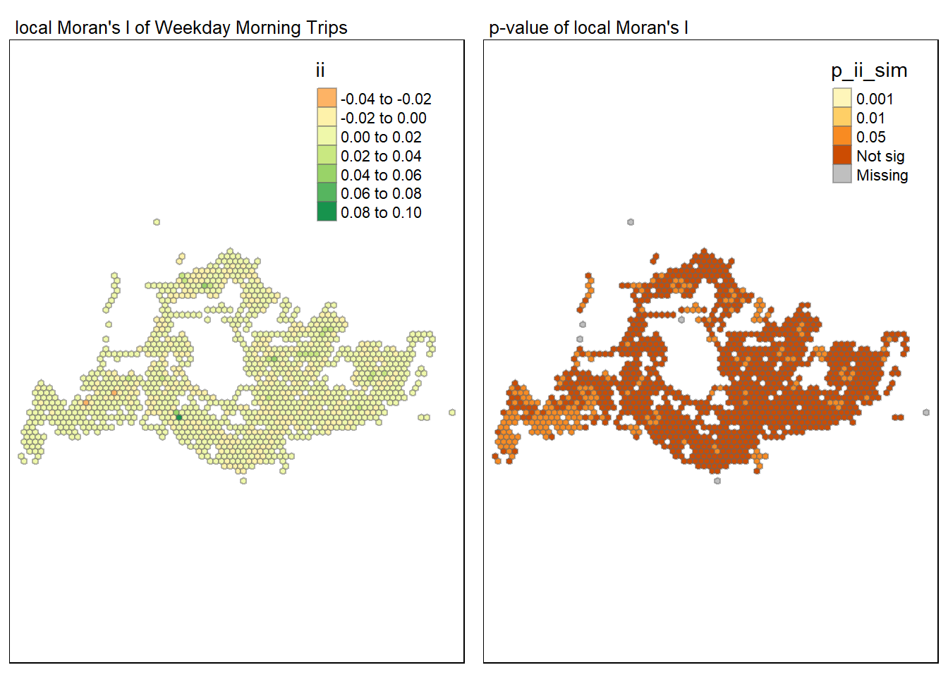
The image shows two side-by-side maps representing the Local Moran’s I results for weekday morning bus trips in Singapore. The left map displays the Local Moran’s I values with a color gradient where darker greens indicate higher positive autocorrelation, suggesting clusters of high trip volumes, and lighter greens to yellows represent areas with lower or negative autocorrelation, indicating either no significant clustering or potential outliers. The right map shows the p-values associated with these Local Moran’s I statistics. Darker browns represent more statistically significant values (strong evidence of spatial clustering or dispersion), and lighter colors represent less significant values. Areas marked as “Not sig” indicate a lack of significant spatial autocorrelation, while “Missing” denotes data that might be unavailable or excluded from the analysis.
lisa_wdm_sig <- lisa_wdm  %>%
  filter(p_ii_sim < 0.05)
tmap_mode("plot")
tm_shape(lisa_wdm) +
  tm_polygons() +
  tm_borders(alpha = 0.5) +
tm_shape(lisa_wdm_sig) +
  tm_fill("mean") +
  tm_borders(alpha = 0.4)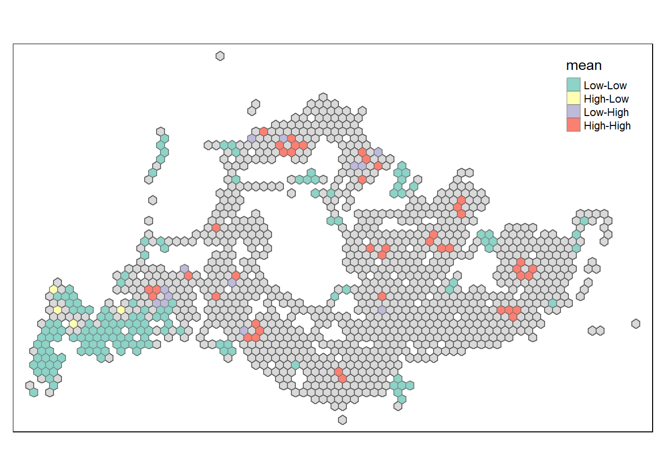
The code calculates LISA for weekday_afternoon_trips, providing Local Moran’s I values to detect spatial patterns like clusters or isolated points for each bus stop.
lisa_wda <- wm_idw %>%
  mutate(local_moran = local_moran(
    weekday_afternoon_trips, nb, wts, nsim = 99, zero.policy = TRUE),
         .before = 1) %>%
  unnest(local_moran)
The LISA map for weekday morning bus trips in Singapore illustrates spatial clusters of similar values. Hexagons marked as “High-High” indicate clusters where bus stops with high trip volumes are surrounded by others with similarly high volumes, likely reflecting central or busy areas with strong demand for bus services. Conversely, “Low-Low” clusters represent areas with uniformly low trip volumes, possibly less urbanized or residential zones with lower bus usage. “Low-High” and “High-Low” hexagons could indicate outliers where a bus stop has a contrasting number of trips compared to its neighbors, such as a busy stop in a generally quiet area or vice versa. These patterns suggest targeted areas for potential service improvements or adjustments to meet passenger demand effectively in Singapore’s urban transport landscape.
The first map could show the Local Moran’s I values for weekday afternoons, indicating areas where bus stops with similar trip counts are located near each other, while the second map would represent the p-values, highlighting the areas where the spatial patterns are statistically significant.
tmap_mode("plot")
map1 <- tm_shape(lisa_wda) +
  tm_fill("ii") +
  tm_borders(alpha = 0.5) +
  tm_view(set.zoom.limits = c(6,8)) +
  tm_layout(main.title = "local Moran's I of Weekday Afternoon Trips",
            main.title.size = 0.8)

map2 <- tm_shape(lisa_wda) +
  tm_fill("p_ii_sim",
          breaks = c(0, 0.001, 0.01, 0.05, 1),
              labels = c("0.001", "0.01", "0.05", "Not sig")) +
  tm_borders(alpha = 0.5) +
  tm_layout(main.title = "p-value of local Moran's I",
            main.title.size = 0.8)

tmap_arrange(map1, map2, ncol = 2)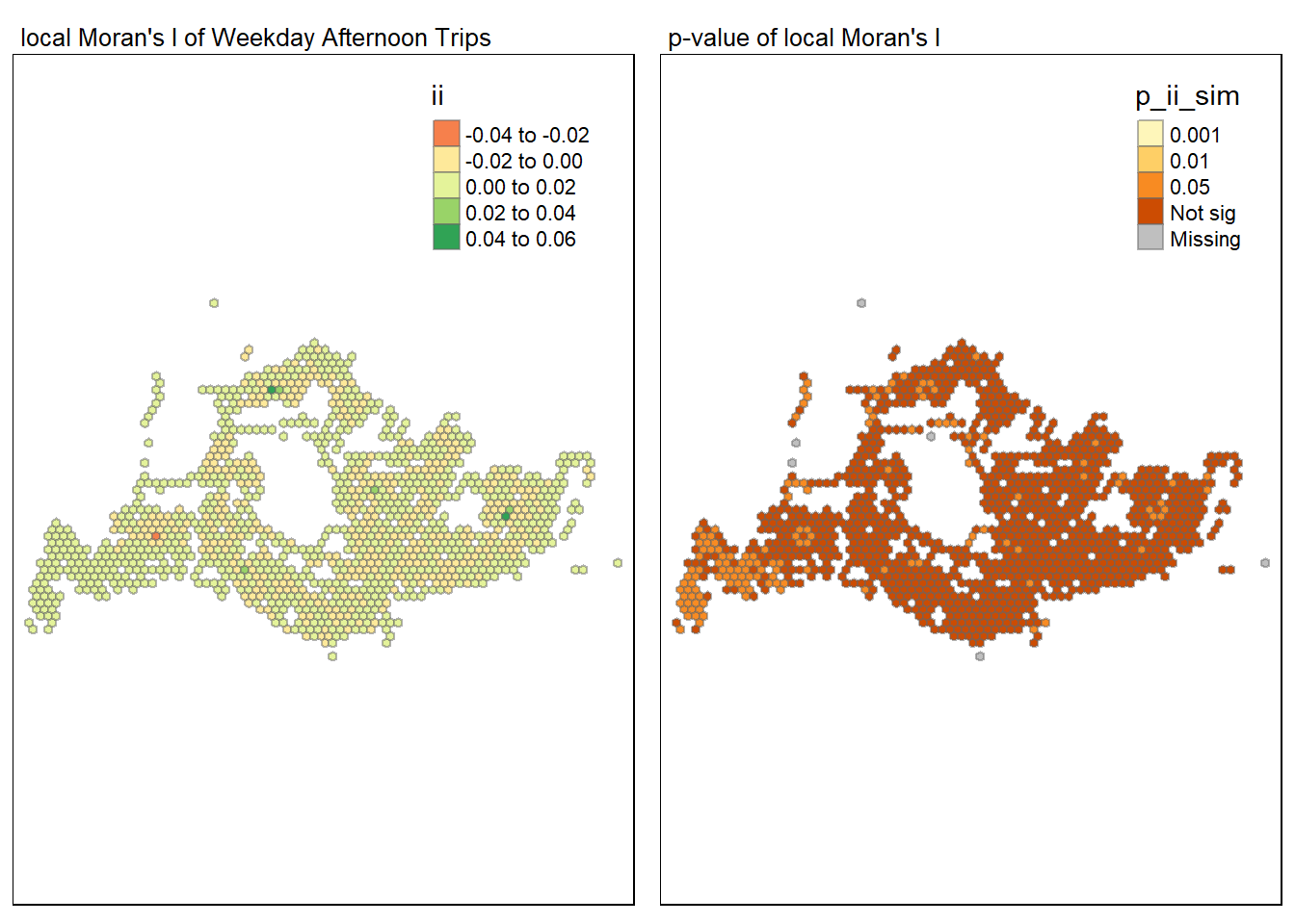
The LISA map for weekday afternoon bus trips in Singapore shows various spatial clusters indicating how bus trip volumes are distributed. The “High-High” areas (red) suggest pockets of high ridership likely around key commercial districts or busy residential areas where people are heading home or to after-work activities. The “Low-Low” regions (light blue) might correspond to less active parts of the city during the afternoon, such as business districts winding down or quieter residential areas. The presence of “Low-High” and “High-Low” outliers could indicate specific stops that defy the general trend of their surroundings, such as a busy stop in a generally quiet area or a quiet stop in a busy area. These insights could help optimize bus service allocation for the afternoon commute in Singapore.
lisa_wda_sig <- lisa_wda  %>%
  filter(p_ii_sim < 0.05)
tmap_mode("plot")
tm_shape(lisa_wda) +
  tm_polygons() +
  tm_borders(alpha = 0.5) +
tm_shape(lisa_wdm_sig) +
  tm_fill("mean") +
  tm_borders(alpha = 0.4)
For weekend_morning_trips, the script performs LISA, yielding Local Moran’s I values that highlight spatial correlations, pinpointing areas of similar trip densities.
lisa_wem <- wm_idw %>%
  mutate(local_moran = local_moran(
    weekend_morning_trips, nb, wts, nsim = 99, zero.policy = TRUE),
         .before = 1) %>%
  unnest(local_moran)
A similar pair of maps for weekend mornings would identify clusters or outliers of bus trip volumes and the significance of these patterns, showing how spatial correlations may differ from weekdays due to different travel behaviors.
tmap_mode("plot")
map1 <- tm_shape(lisa_wem) +
  tm_fill("ii") +
  tm_borders(alpha = 0.5) +
  tm_view(set.zoom.limits = c(6,8)) +
  tm_layout(main.title = "local Moran's I of Weekend Morning Trips",
            main.title.size = 0.8)

map2 <- tm_shape(lisa_wem) +
  tm_fill("p_ii_sim",
          breaks = c(0, 0.001, 0.01, 0.05, 1),
              labels = c("0.001", "0.01", "0.05", "Not sig")) +
  tm_borders(alpha = 0.5) +
  tm_layout(main.title = "p-value of local Moran's I",
            main.title.size = 0.8)

tmap_arrange(map1, map2, ncol = 2)
The LISA map for weekend mornings in Singapore indicates areas where departure activity is concentrated. “High-High” clusters point to departure stops with a high volume of trips, likely in areas with weekend attractions or key residential zones from where people start their weekend outings. “Low-Low” areas signify stops with fewer departures, which could correlate with less active zones during weekend mornings.
lisa_wem_sig <- lisa_wem  %>%
  filter(p_ii_sim < 0.05)
tmap_mode("plot")
tm_shape(lisa_wem) +
  tm_polygons() +
  tm_borders(alpha = 0.5) +
tm_shape(lisa_wem_sig) +
  tm_fill("mean") +
  tm_borders(alpha = 0.4)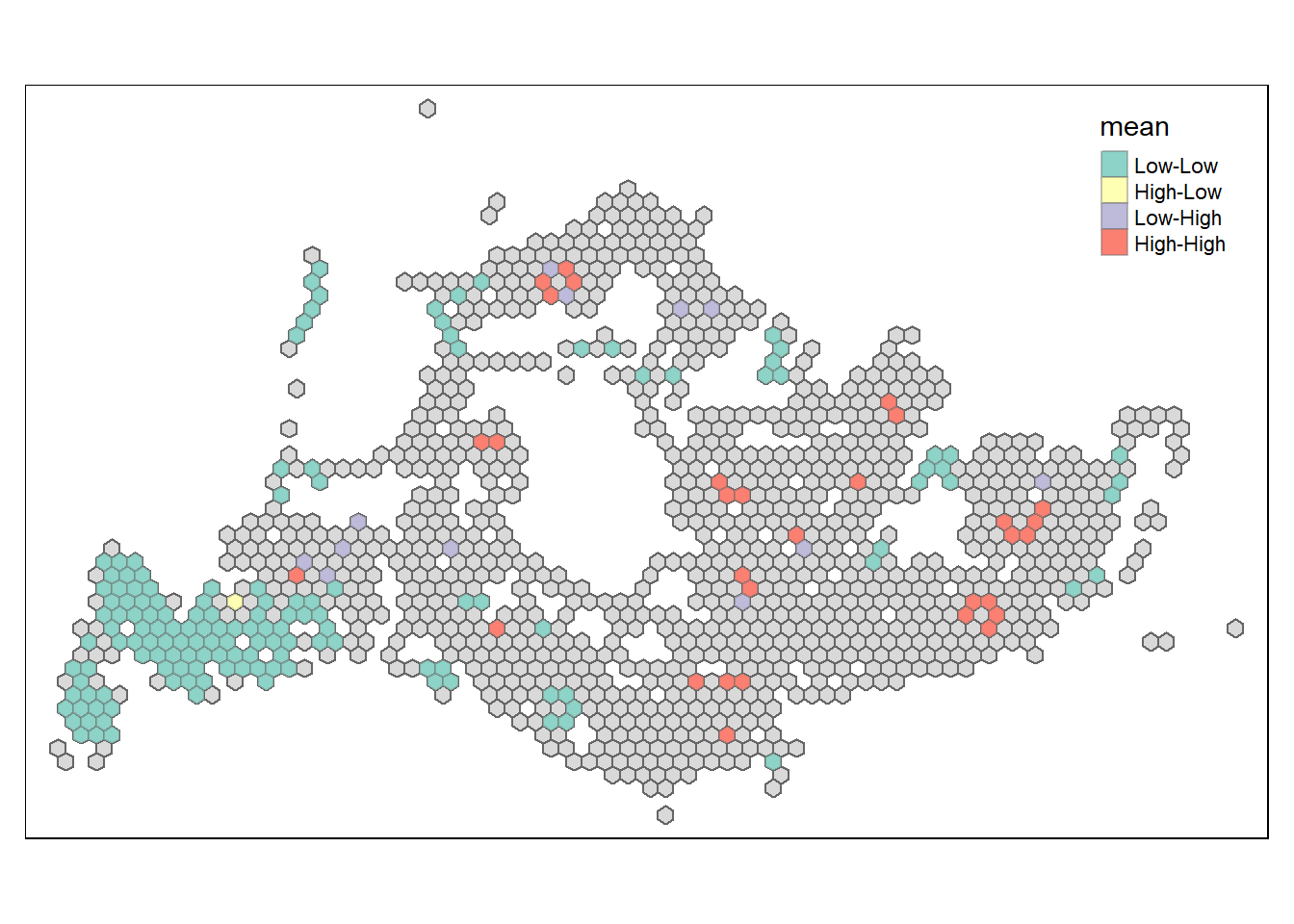
The analysis applies LISA to weekend evening trips, generating Local Moran’s I statistics that reveal the geographic distribution of trip volumes, identifying potential clusters.
lisa_wee <- wm_idw %>%
  mutate(local_moran = local_moran(
    weekend_evening_trips, nb, wts, nsim = 99, zero.policy = TRUE),
         .before = 1) %>%
  unnest(local_moran)
For weekend evenings, the maps would again display the Local Moran’s I values and their significance, illustrating the spatial distribution of bus trip volumes during leisure times, which might show a different pattern compared to mornings and afternoons.
tmap_mode("plot")
map1 <- tm_shape(lisa_wee) +
  tm_fill("ii") +
  tm_borders(alpha = 0.5) +
  tm_view(set.zoom.limits = c(6,8)) +
  tm_layout(main.title = "local Moran's I of Weekend Evening Trips",
            main.title.size = 0.8)

map2 <- tm_shape(lisa_wee) +
  tm_fill("p_ii_sim",
          breaks = c(0, 0.001, 0.01, 0.05, 1),
              labels = c("0.001", "0.01", "0.05", "Not sig")) +
  tm_borders(alpha = 0.5) +
  tm_layout(main.title = "p-value of local Moran's I",
            main.title.size = 0.8)

tmap_arrange(map1, map2, ncol = 2)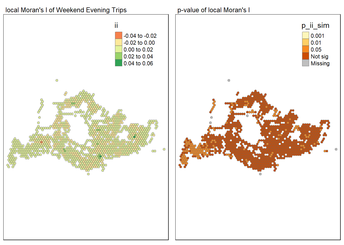
The LISA map for weekend evening bus trips in Singapore displays “High-High” clusters, indicating areas with a high volume of bus departures, possibly reflecting popular social or recreational destinations active during weekend evenings. “Low-Low” clusters suggest areas with uniformly low departure volumes, which could be residential zones with less outbound activity at this time. The presence of both “High-Low” and “Low-High” areas signifies spots where departure volumes significantly differ from their surroundings, pointing to unique transit patterns. These findings can guide the optimization of bus services to meet the distinct travel demands of weekend evenings in Singapore.
lisa_wee_sig <- lisa_wee  %>%
  filter(p_ii_sim < 0.05)
tmap_mode("plot")
tm_shape(lisa_wee) +
  tm_polygons() +
  tm_borders(alpha = 0.5) +
tm_shape(lisa_wee_sig) +
  tm_fill("mean") +
  tm_borders(alpha = 0.4)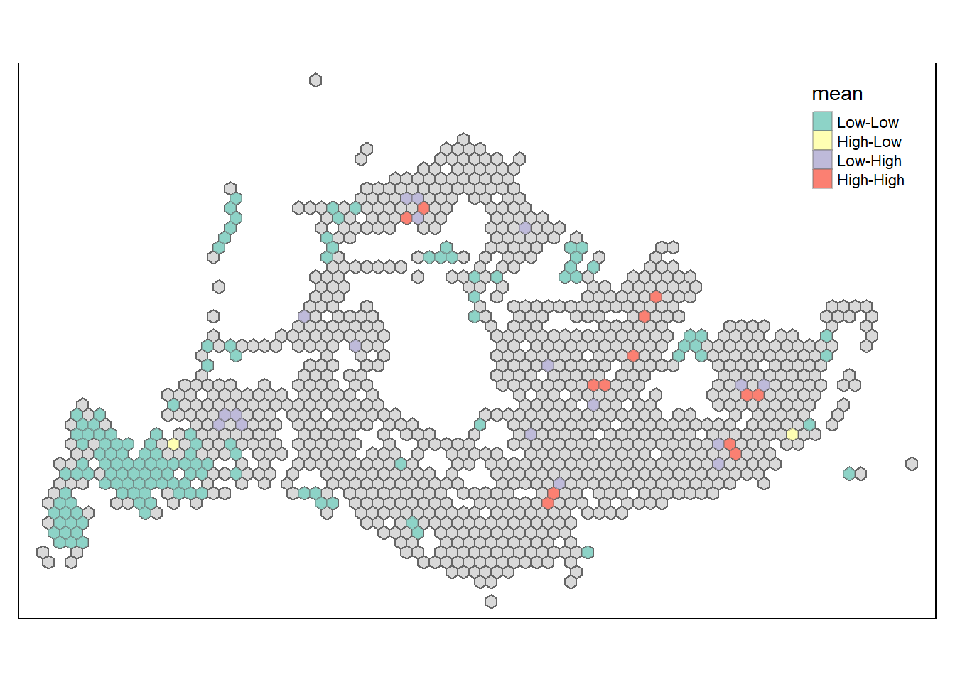
The code provided is removing a list of data frames and variables and cleaning R environment.
rm(lisa_wda, lisa_wda_sig, lisa_wdm, lisa_wdm_sig, lisa_wee, lisa_wee_sig, lisa_wem, lisa_wem_sig, map1, map2, nb, wm_ad, wm_fd, wm_idw, dists)5.Emerging Hot Spot Analysis
Due to technical difficulties, Task 3 has not been fully completed as planned.
5.1Mitigating the Data Gap
5.1.1Supplementary Data for Weekday Trips
The R code snippet is designed to prepare a comprehensive dataset for analyzing weekday bus trips. It begins by creating a data frame of all 24 hours in a day, which it then cross-references with a list of unique bus stop codes to ensure there is an hourly record for each stop. Next, it merges this exhaustive hourly schedule with the existing trip data, keeping all the hourly records even if they don’t match any original data (all.x = TRUE). Finally, it addresses any missing trip data resulting from the merge by replacing NA values with zeros, thus ensuring that the dataset reflects zero trips during hours where no data was recorded, maintaining the integrity of the time series.
# Create a complete set of hours for each ORIGIN_PT_CODE
hours <- data.frame(TIME_PER_HOUR = 0:23)
origin_pt_codes <- unique(weekday_trips$ORIGIN_PT_CODE)
complete_hours <- expand.grid(ORIGIN_PT_CODE = origin_pt_codes, TIME_PER_HOUR = hours$TIME_PER_HOUR)

# Merge the complete set of hours with the original data
# and replace NA values with zero
weekday_trips_complete <- merge(complete_hours, weekday_trips, by = c("ORIGIN_PT_CODE", "TIME_PER_HOUR"), all.x = TRUE)
weekday_trips_complete$TRIPS[is.na(weekday_trips_complete$TRIPS)] <- 0
The code merges the busstop_hex dataframe, which likely contains hexagonally binned bus stop locations, with the weekday_trips_complete dataframe, matching them on the bus stop number and origin point code to integrate complete weekend trip data into the spatial hex grid.
weekday_trips_hex <- busstop_hex %>%
  inner_join(weekday_trips_complete, by = c("BUS_STOP_N" = "ORIGIN_PT_CODE"))
The code aggregates the total number of bus trips for each hexagonal cell and each hour of the weekend by summing up the trip counts while omitting any missing values (NA).
weekday_trips_summary <- weekday_trips_hex %>%
  group_by(hex_id, TIME_PER_HOUR) %>%
  summarise(total_trips = sum(TRIPS, na.rm = TRUE))
5.1.2Supplementary Data for Weekend/Holiday Trips
The provided R code constructs a complete time-series dataset for bus trips by ensuring that each bus stop has trip data for every hour of the day. It first generates a full list of hourly time slots and matches them with each unique bus stop code to create a comprehensive grid. This grid is then merged with the existing trip data, filling in any gaps where no trips were recorded with zeros. The result is a dataset with no missing time points, allowing for accurate time-series analysis for each bus stop across the weekday hours.
# Create a complete set of hours for each ORIGIN_PT_CODE
origin_pt_codes <- unique(weekend_trips$ORIGIN_PT_CODE)
complete_hours <- expand.grid(ORIGIN_PT_CODE = origin_pt_codes, TIME_PER_HOUR = hours$TIME_PER_HOUR)

# Merge the complete set of hours with the original data
# and replace NA values with zero
weekend_trips_complete <- merge(complete_hours, weekend_trips, by = c("ORIGIN_PT_CODE", "TIME_PER_HOUR"), all.x = TRUE)
weekend_trips_complete$TRIPS[is.na(weekend_trips_complete$TRIPS)] <- 0
The code merges the busstop_hex dataframe, which likely contains hexagonally binned bus stop locations, with the weekend_trips_complete dataframe, matching them on the bus stop number and origin point code to integrate complete weekend trip data into the spatial hex grid.
weekend_trips_hex <- busstop_hex %>%
  inner_join(weekend_trips_complete, by = c("BUS_STOP_N" = "ORIGIN_PT_CODE"))
The code aggregates the total number of bus trips for each hexagonal cell and each hour of the weekend by summing up the trip counts while omitting any missing values (NA).
weekend_trips_summary <- weekend_trips_hex %>%
  group_by(hex_id, TIME_PER_HOUR) %>%
  summarise(total_trips = sum(TRIPS, na.rm = TRUE))
5.1.3Importing Hexagon Layer
The code chunk below uses st_read() from the sf package to read the spatial data we created previously.
hex_grid_sf <- st_read(dsn = "data/geospatial",
                 layer = "hex_layer")
Reading layer `hex_layer' from data source
`D:\KathyChiu77\ISSS624\Take-home Ex\Take-home Ex 1\data\geospatial'
using driver `ESRI Shapefile'
Simple feature collection with 1237 features and 2 fields
Geometry type: POLYGON
Dimension: XY
Bounding box: xmin: 3392.771 ymin: 26148.77 xmax: 48714.77 ymax: 53315.43
Projected CRS: SVY21 / Singapore TM5.2Creating a Time Series Cube
The code transforms the summarized weekday trips data into a space-time cube using the as_spacetime() function. It combines the weekday_trips_summary, which contains aggregated trip data by hour and hexagon, with the spatial information in hex_grid_sf, specifying hex_id as the location identifier and TIME_PER_HOUR as the temporal dimension. This results in a structured dataset that facilitates the analysis of trip volumes over time within the spatial framework of the hexagonal grid.
weekday_trips_st <- as_spacetime(weekday_trips_summary, hex_grid_sf,
                      .loc_col = "hex_id",
                      .time_col = "TIME_PER_HOUR")
The function is_spacetime_cube(weekday_trips_st) is used to check if the object weekday_trips_st is correctly formatted as a space-time cube. It returns a logical value: TRUE if weekday_trips_st is a valid space-time cube, and FALSE otherwise.
is_spacetime_cube(weekday_trips_st)[1] TRUEThe code transforms the summarized weekday trips data into a space-time cube using the as_spacetime() function. It combines the weekend_trips_summary, which contains aggregated trip data by hour and hexagon, with the spatial information in hex_grid_sf, specifying hex_id as the location identifier and TIME_PER_HOUR as the temporal dimension.
weekend_trips_st <- as_spacetime(weekend_trips_summary, hex_grid_sf,
                      .loc_col = "hex_id",
                      .time_col = "TIME_PER_HOUR")
The function is_spacetime_cube(weekend_trips_st) is used to check if the object weekend_trips_st is correctly formatted as a space-time cube. It returns a logical value: TRUE if weekday_end_st is a valid space-time cube, and FALSE otherwise.
is_spacetime_cube(weekend_trips_st)[1] TRUEReference
https://desktop.arcgis.com/zh-cn/arcmap/latest/tools/spatial-statistics-toolbox/h-whyhexagons.htm
